PingPlot
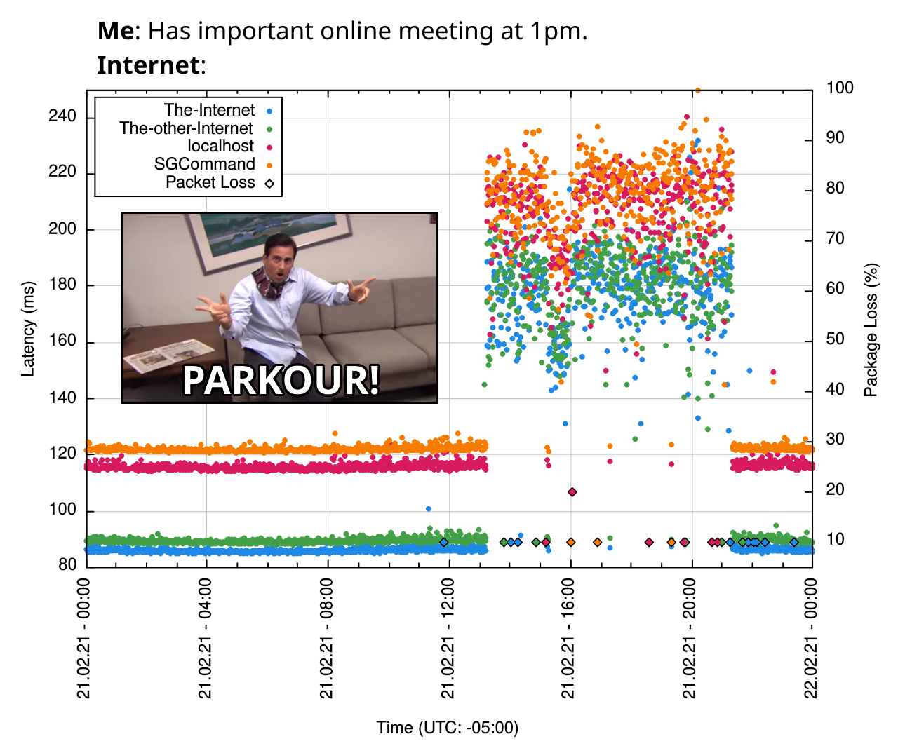
Want to create memes graphs of your network connectivity? Ping and plot away:
Getting started
• Configuration
• Roadmap
## Getting started
> **DISCLAIMER:** The author accepts no responsibility or liability for the use of this software. A high frequency of `ICMP` requests could be seen as `DoS` attack. Please ensure you have permission to ping the target servers!
In the default configuration a server will be pinged `10` times with `0.2s` between each ping every `60s`.
This tool requires `net-tools` (if not using a docker container) and `gnuplot` installed on the system.
1. Configure the servers to be pinged and their label in the graph's legend in the [`servers.env`](servers.env) file:
```
:
0.0.0.0:localhost
my_server.x:my-server
```
Note that `gnuplot` will interprets some characters (such as `_` underscore) in `` as mathematical notation.
2. Run [`./files/inet_stat.sh`](files/inet_stat.sh) or start a docker container which includes the script with `docker-compose up`
3. Plot the data with [`./plotter/plot.sh`](plotter/plot.sh)
## Configuration
### Plot
The `./plotter/plot.sh` script offers a variety of options to control the output of the graph.
```
usage: SERVER:LABEL [...]
[--file|-f CSV_FILE] [--limit-y|-l Y_MAX] [--time-zone|-t UTC_HOURS]
[--start-date|-S DATE] [--end-date|-E DATE] [--show-hours|-H HOURS]
[--align-legend|-a POSITION]
```
Examples:
```bash
./plotter/plot.sh example.local:example 0.0.0.0:localhost --limit-y 100 --show-hours 5 --end-date "2021-03-03 20:11" --time-zone -5
./plotter/plot.sh example.local:example 0.0.0.0:localhost -S 2021-03-02 -E 2021-03-03 -f data.csv
```
Run [`./plotter/plot.sh --help`](plotter/plot.sh) for details.
### Ping
The script `./files/inet_stat.sh` which pings the target servers and records the data can be configured via environment variables:
```bash
# space seperated list of servers (takes precedence over servers.env)
SERVERS="127.0.0.1
0.0.0.0
localhost"
# sets the cycle at which servers are pinged `sleep $CYCLE` [default: 60s]
CYCLE=60s
# sets the amount of times servers are pinged on each cycle [default: 10]
PING_COUNT=10
# sets the output file name [default: ping.csv]
OUTPUT_FILE=ping.csv
# sets the directory path of the output file [default: ./data]
OUTPUT_PATH=./data
# sets the servers.env file path [default: ./servers.env]
SERVER_FILE=./servers.env
# changes the Epoch columns format `date $DATE_FORMAT`, e.g. -Iseconds, [default: +%s]
# ONLY change if you want to use the csv file for another purpose
# any change from the default will prevent plotting using ./plotter/plot.sh
DATE_FORMAT=+%s
```
These can also be set in the `docker-compose.yml` in the `environment` section.
### Latency Data
Latency data is saved in [`data/ping.csv`](data/ping.csv). You can add your own data as long as it has the following format (first line has the column names):
```csv
Epoch,Server,PacketLoss,Min,Average,Max,Deviation
1613501993,localhost,0%,87.519,89.085,91.4,1.106
1613501995,0.0.0.0,0%,120.358,122.399,126.254,1.712
1613501997,127.0.0.1,0%,113.125,116.473,125.609,3.311
```
Viewed in table form:
| *(UNIX)* Epoch | Server | PacketLoss | Min | Average | Max | Deviation |
|------------|-----------|------------|---------|---------|---------|-----------|
| 1613501993 | localhost | 0% | 87.519 | 89.085 | 91.4 | 1.106 |
| 1613501995 | 0.0.0.0 | 0% | 120.358 | 122.399 | 126.254 | 1.712 |
| 1613501997 | 127.0.0.1 | 0% | 113.125 | 116.473 | 125.609 | 3.311 |
## Roadmap
* Record each server in a separate file to be able to have `gnuplot` draw lines between each point.
* Record into a new `csv` each day and have `./plotter/plot.sh` temporarily merge these based on the start and end date to be plotted. This should cut down on plotting time as `gnuplot` will not have to read large files anymore.
* Add a flag to keep the merged file permanently.
* Automated plotting
* Directly in the Docker Container and server via web server
* Move the plotting into a web interface